XRS Academy
Practical knowledge and insights on XRF analysis
Why XRF calibrations often include more elements than you actually report.
Many XRF users wonder why a calibration method sometimes includes elements that are never reported in routine analysis. At first glance, this seems unnecessary work, but in reality, it is necessary to obtain accurate and stable results.
This is because in an XRF analysis, the emitted energies of all elements present in the sample can influence each other. The intensities of one element can enhance the intensities of another element while its own energy is absorbed. In addition, certain peaks in the spectra can overlap with the peak of the element of interest.
These so-called matrix effects can be compensated by mathematics in the XRF method, however, it still requires the data to do so. Therefore, when calibrating an XRF method, it is important to include all elements that might vary in concentration, even if they are not reported.
Let’s have a closer look at the phenomenon of absorption and enhancement:
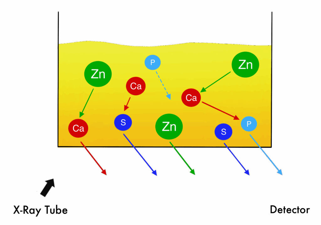
When a sample is irradiated with X-rays, all elements present are excited and emit characteristic X-rays. The X-rays emitted by heavier elements have higher energies and can travel all the way through the sample to reach the detector. In contrast, X-rays from lighter elements are more easily absorbed by the sample matrix, meaning that only those generated near the sample surface will be detected. As these characteristic X-rays travel through the sample, they may interact with other elements. If the energy of the characteristic X-rays is higher than the binding energy of another element’s inner-shell electrons, it can excite that element. In this process, the original X-ray is absorbed and therefore no longer detected. Its energy is transferred to enhance the intensity of the element it interacted with. As a result, the original element will show a negative bias in the measured results, while the element that is enhanced will exhibit a positive bias.
Practical example:
A practical example can be found in the analysis of lubricating oils where Zn, Ca, S and P are typically present together. X-rays generated by one element can be partially absorbed or enhanced by others, meaning measured intensities no longer scale linearly with concentrations.
In a first step we calculate the concentrations only using the basic linear calibration equation:
Celement = Delement + Eelement x Relement
C = concentration
D = intercept
E = slope
R = intensity of the element of interest
In this example this gives us:
Zn = 0.0976%
Ca = 0.1913%
S = 0.4857%
P = 0.0975%
At this stage, each element is effectively treated as if it were present alone in the sample. The instrument converts count rates into concentrations using linear calibration parameters, without taking into account interactions between elements. For simple matrices this approximation may be acceptable, but in multi-element systems such as lubricating oils, it introduces significant error.
In a second step we correct for the matrix effects. Concentrations are corrected using influence coefficients (α values) that describe how strongly elements affect each other. The equation including these correction factors can be described as follows:
Ci = Di + Ei x Ri x (1 + Σj=1 α i,j x Cj)
Ci = concentration of element i
Di = intercept of element i
Ei = slope of element i
Ri = intensity of element i
α i 🠢 j = influence coefficient of element j on element i
Cj = concentration of element j
In our example this translates to:
C Zn corrected = C Zn initial x (1 + α Zn 🠢 Zn x CZn + α Ca 🠢 Zn x CCa + α S 🠢 Zn x CS + α P 🠢 Zn x CP)
C Ca corrected = C Ca initial x (1 + α Zn 🠢 Ca x CZn + α Ca 🠢 Ca x CCa + α S 🠢 Ca x CS + α P 🠢 Ca x CP)
C P corrected = C P initial x (1 + α Zn 🠢 P x CZn + α Ca 🠢 P x CCa + α S 🠢 P x CS + α P 🠢 P x CP)
C S corrected = C S initial x (1 + α Zn 🠢 S x CZn + α Ca 🠢 S x CCa + α S 🠢 S x CS + α P 🠢 S x CP)
After applying these corrections we get following results in the second iteration:
Zn = 0.1221%
Ca = 0.2213%
S = 0.5123%
P = 0.1003%
As you can see, the influence of these correction factors is very noticeable and in order to be able to calculate them, we also need the concentrations of the other elements that are present in the sample.
Because the correction on one element depends on the concentrations of the others, the calculation is iterative. In a third step the newly corrected concentrations are reinserted into the correction formula to refine the results.
Zn = 0.1248%
Ca = 0.2236%
S = 0.5147%
P = 0.1007%
After the third iteration, the results are stable and further corrections are negligible.
So why do we sometimes have to include more elements than we actually report?
Compared to the initial values, Zn was underestimated by nearly 25% relative, Ca by 16%, S by 6% and P by 3%.
| 1st iteration | 2nd iteration | 3rd iteration |
| Zn = 0.0976% | Zn = 0.1221% | Zn = 0.1248% |
| Ca = 0.1913% | Ca = 0.2213% | Ca = 0.2236% |
| S = 0.4857% | S = 0.5123% | S = 0.5147% |
| P = 0.0975% | P = 0.1003% | P = 0.1007% |
This example clearly demonstrates that elements analysed by XRF spectrometry do not behave independently. This is why XRF calibrations often include more elements than are actually reported. Even if the primary focus is on Zn, the other varying elements Ca, P and S must be included to properly correct for matrix effects. Without these additional elements in the calibration, the instrument cannot apply the necessary corrections, and the results will systematically deviate.
Reach Out To Us
Do you want to reach out for more information or see how we can help you? Reach out to us by clicking on the button below.